10. Tools Plugins
The following plugins contain utilities for image manipulation.
The plugins are described in the following sections using the order presented on the
Plugins > GDSC SMLM > Tools
menu.
10.1. Smooth Image
Provides a filter plugin for smoothing an image (see Table 10.1).
|
|
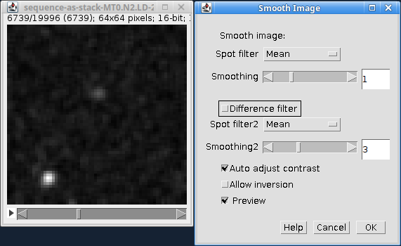
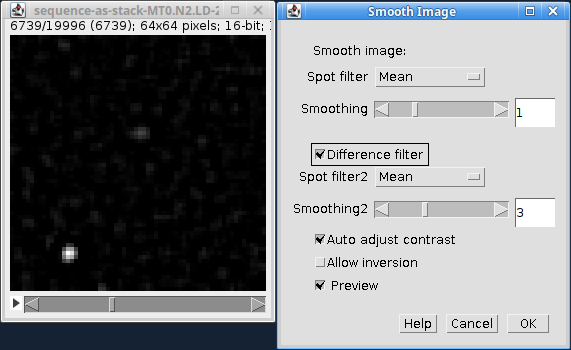
The filter uses the same methods as the Peak Fit plugin for identifying local maxima. However only a single or difference filter is available (no Jury filter) so that a single dialog can display all the options. A single filter applies a single smoothing operation to the image. A difference filter applies two smoothing operations and the second smoothed image is subtracted from the first. This produces a difference-of-smoothing image. As can be seen by comparing Table 10.1 (A) and (B), the difference filter is beneficial when there is a variable background across the image. The filter reduces the contribution the background has to the brightness of the spots by performing local contrast enhancement.
The following algorithms are available:
Algorithm |
Description |
|---|---|
Mean |
Compute the mean in a square region. The region can be any size as the final edge pixels are given a weight using the region width. |
Block mean |
Compute the mean in a square region. The region is rounded to integer pixels. |
Circular mean |
Compute the mean in an approximate circular region. The circle is drawn using square pixels. To see the circle mask use |
Gaussian |
Perform Gaussian convolution. The convolution kernel standard deviation is set to the The total region width around each point that is used will be 2n+1 with \(n=\lceil 2.8\sigma \rceil\) where \(\lceil x \rceil\) is the ceiling function. |
Median |
Compute the median in a square region. The region is rounded to integer pixels. |
The following additional parameters can be set:
Parameter |
Description |
|---|---|
Auto adjust contrast |
Adjust the contrast of the preview using the min and max value of the smoothed image. |
Allow inversion |
Allow the second smoothing parameter of a difference filter to be smaller that the first. This will create an inverted image where bright spots are dark and possibly surrounded by a ring. If not enabled the plugin raises an error and will disable an active current preview. |
Preview |
Preview the smoothing filter on the image. |
Use the Preview button to see the effect of smoothing. If you click OK the plugin will perform smoothing on the entire stack or optionally just the current frame.
10.1.1. Smoothing within the Peak Fit plugin
Note that the Peak Fit plugin calculates the smoothing window size using a factor of the PSF width. This can result in a non-integer value. Algorithms that require integer window sizes (e.g. block mean, median) have the window size rounded down to the nearest integer to avoid over smoothing.
Most images analysed within the Peak Fit plugin will use a filter size less than 4 due to the small size of the PSF from single molecule microscopy.
10.2. Binary Display
Switches an image to binary (white/black) to allow quick visualisation of localisations.
The SMLM plugins contain several methods for generating an image. Often images are created with a large difference in value for pixels that contain localisations. The difference can be so great that some localisations are not visible. The Binary Display plugin converts all non-zero pixels to the value 1. This allows the user to see any pixel that contains any level of localisation. This mode may be useful for drawing regions of interest (ROIs) around dense sections of localisations.
The plugin does not modify the image data. The display range for the current frame is set to use zero for the minimum and the maximum is set to the smallest non-zero value in the data, effectively clipping the non-zero pixels to the highest value in the current look-up table. Note that this plugin shows pixels with a value above zero. Negative pixel values in 32-bit images are effectively set to zero. The display can be reset using the Reset Display plugin.
10.3. Reset Display
Resets a binary image generated by Binary Display back to the standard display.
The display is reset to the standard display range. For 8-bit images this is [0, 255]. For 16-bit or 32-bit images the range is [min, max]. Note that the Binary Display plugin saves the [min, max] before updating the values for a binary display. The saved values are used if available. This will only work for stack images if the user remains at the same slice position. Moving to a new slice and back will delete the information used to reset the image.
The display can be manually reset using Image > Adjust > Brightness/Contrast ....
10.4. Pixel Filter
Perform filtering to replace hot pixels from an image.
The Pixel Filter is a simple plugin that will replace pixels with the mean of the surrounding region if they are more than N standard deviations from the mean. The filter is designed to remove outlier (hot) pixels that are much brighter then their neighbour pixels. These pixels will be identified as candidate maxima by the Peak Fit plugin although they are not suitable for Gaussian fitting.
The filter operates on the currently selected image. The preview option allows the results of the filter to be viewed before running the filter on the current frame or optionally the entire image stack.
The filter uses a cumulative sum and sum-of-squares lookup table to compute the region mean and standard deviation. This allows fast computation in constant time regardless of the size of the neighbourhood region.
The following parameters can be set:
Parameter |
Description |
|---|---|
Radius |
The radius of the square neighbourhood region. |
Error |
The number of standard deviations above the mean that identifies a hot pixel. |
Preview |
Preview the filter on the image. The number of pixels replaced will be shown in the dialog. |
10.5. Noise Estimator
Estimates noise in an image. This plugin can be used to compare noise estimation methods. Note that estimating the noise in an image is important when setting the signal-to-noise ratio (SNR) for use in filtering localisation fitting results.
When loaded the plugin provides a plot of the noise estimate of the next 100 frames of a stack (from the current frame) as shown in Figure 10.1. Two noise estimation methods can be chosen (see table below). Changing an estimation method will dynamically update the noise plot.
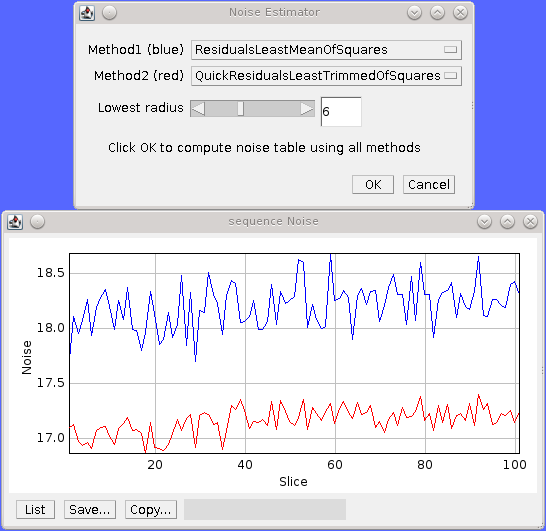
Fig. 10.1 Noise Esimator plugin dialog and the noise plot for the next 100 frames in the image.
Method1 is shown in blue, Method2 is shown in red.
If you click OK the plugin will compute all the estimation methods for the entire stack (or optionally just the current frame) and display the results in a table.
The following noise methods are available:
Method |
Description |
|---|---|
All Pixels |
The standard deviation of the pixels. |
Lowest Pixels |
The standard deviation of a box region around the lowest intensity pixel in the image. The box region can be adjusted using the |
Residuals Least Median Of Squares |
Calculate the median of the residuals. Then use this to estimate the standard deviation of the residuals. |
Residuals Least Trimmed Square Estimator |
Square the residuals. Sum the smallest half of the squared residuals. Then use this to estimate the standard deviation of the residuals. (This is insensitive to high intensity pixels). |
Residuals Least Mean Square Estimator |
Calculate the standard deviation of the residuals. |
Quick Residuals Least Median Of Squares |
As before but ignore pixels on the image boundary. |
Quick Residuals Least Trimmed Square Estimator |
As before but ignore pixels on the image boundary. |
Quick Residuals Least Mean Square Estimator |
As before but ignore pixels on the image boundary. |
10.5.1. Image Residuals
The residuals of an image are calculated for each pixel using the total difference to the 4n connected pixels. These are normalised so that the sum of the residuals squared is the same as the sum of the image pixels squared. Comparing each pixel to its neighbours provides a robust method of estimating noise if the underlying signal is adequately sampled. Variations between neighbour pixels are expected to be small, consequently large variations indicate high noise.
All the image residuals methods are based on the “Least trimmed square” robust estimator described in:
P. Rousseeuw and A. Leroy
Robust Regression and Outlier Detection
New York: Wiley, 1987
10.5.2. Noise Estimation within the Peak Fit Plugin
The fitting code in the Peak Fit plugin currently uses the QuickResidualsLeastMeanOfSquares. This method is more stable than using the standard deviation of the image pixels since large variations around the high intensity localisations are smoothed by using the image residuals.
The noise estimation method can be changed in the Peak Fit plugin by holding the Shift or Alt key down when running the plugin to see the extra options.
10.6. Background Estimator
Estimate the background in a region of an image. The Background Estimator plugin analyses the pixels within a region marked on the image. A thresholding method is applied to the data to determine background pixels using a global histogram. The standard deviation of the background pixels and all pixels is computed as a noise estimate. The background is the mean of the background pixels. If the fraction of background pixels is below a threshold then the mean background is computed using all the data; otherwise the background pixels are used. For reference a background level is computed using a percentile of the data in the region and using a noise estimation method on all the data.
The following parameters can be specified:
Parameter |
Description |
|---|---|
Percentile |
The percentile to compute the background using all the pixel data as an estimate of the background. Using zero will report the minimum value in the data. |
Noise method |
The noise method to apply using all the pixel data as a global noise estimate. |
Threshold method |
The threshold method used to select the background pixels. |
Fraction |
The fraction of the total region that must be covered by background pixels. If the background region area is below this level then the background mean is computed using all pixels. |
Histogram size |
The size of the histogram to use for the thresholding method. Note: The data is processed as a 32-bit floating point image so the histogram bins can be defined using any bin width. |
The plugin runs in a preview mode where results are displayed on plots for the 100 frames after the current frame in the stack. Changes to parameters result in re-computation of the plots. The Noise plot shows the background noise and global noise estimate. The Background plot shows the threshold computed for background pixels, the mean of the background pixels and the percentile level using all pixels.
Pressing OK in the plugin dialog will create a table of the results. This can be for either the current frame or all frames in the stack. The results table contains all the data from the plots in tabulated form. An additional column IsBackground is set to 1 if the background area was above the configured Fraction and the estimate used only the background pixels; otherwise it is set to 0 indicating the results for the Background and Noise columns are the mean and standard deviation of all the pixels.
10.7. Median Filter
Compute the median of an image, on a per-pixel basis, using a rolling window at set intervals.
Super-resolution image data can contain a low amount of background which affects the performance of fitting routines if it is not constant, for example cell walls may be visible as a change in low level fluorescence over a distance of a few pixels. This uneven background will not be modelled by a fitting routine which assumes the background is constant. Any local gradients in the background can be eliminated by assuming that all real fluorescence over a short time frame will be much higher than the other values for the pixels in the same location. Using the median value for the pixel will approximate the background. This can be subtracted from the image data prior to fitting so that only fluorescent bursts are left for fitting.
The Median Filter plugin will compute the median for each pixel column through the image (i.e. all z positions of the pixel) using a rolling window. The median can be calculated at every pixel or at intervals. In the case of interval calculation then the intermediate points have linearly interpolated medians.
The median image either replaces the input image, or is subtracted from the input image to produce an image with only localisations. A bias offset is added to this image to allow noise to be modelled (i.e. values below zero).
The following parameters can be specified:
Parameter |
Description |
|---|---|
Radius |
The number of pixels to use for the median. The median is calculated using a window of \(2 \times \mathit{radius} + 1\). |
Interval |
The interval between slices to calculate the median. An interval of 1 will produce a true rolling median. Larger intervals will require interpolation for some pixels. |
Block size |
The algorithm is multi-threaded and processes a block of pixels on each thread in turn. Specify the number of pixels to use in a block. Larger blocks will require more memory due to the algorithm implementation for calculating rolling medians. The number of threads is set in |
Subtract |
Subtract the median image from the original image. |
Bias |
If subtracting the median, add a bias to the result image so that negative numbers can be modelled (i.e. when the original image data is lower than the median). |
10.8. Image Background
Produces a background intensity image and a mask from a sample image.
The Image Background plugin is used to generate suitable input for the Create Data plugin. The Create Data plugin creates an image by simulating fluorophores using a distribution. One allowed distribution is the region defined by a mask. The fluorophores are created and then drawn on the background. The background can be an input image. Both the mask and background image can be created from a suitable in vivo image using the Image Background plugin. The purpose would be to simulate fluorophores in a distribution that matches that observed in super-resolution experiments.
The plugin requires that an image is open. The plugin dialog is show in Figure 10.2.
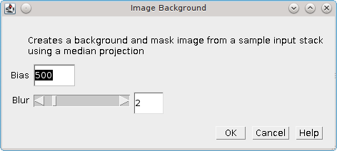
Fig. 10.2 Image background dialog
10.8.1. Image Analysis
The Image Background plugin first computes a median intensity projection of the input image. A Gaussian blur is then applied to the projection to smooth the image. The blur parameter controls the size of the Gaussian kernel.
The bias is subtracted from the blurred image. The bias is an offset that may be added to the pixel values read by the camera so that negative noise values can be observed. It is a constant level that can be subtracted. What remains should be the background level. The bias subtraction can be ignored using a bias of zero.
Two output images are then displayed:
Image |
Description |
|---|---|
Background |
The blurred projection. |
Mask |
The blurred projection subjected to the |
10.9. Overlay Image
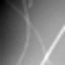
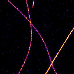
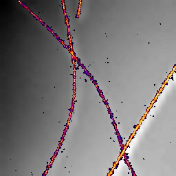
Allow an image to be added as an overlay with a transparent background. Using a transparent background is not possible with the standard ImageJ Image > Overlay > Add image... command.
For example the super-resolution image created from fitting localisations can be overlaid on the average z-projection of the original image to show where the localisations occur (see Table 10.2):
|
The Overlay Image plugin must be run after selecting the image to overlay. The following parameters can be specified:
Parameter |
Description |
|---|---|
Image to add |
Select the image to use as the overlay. The list only shows the images that are valid. Overlay images must be equal or smaller in width and height than the target image. |
X location |
The x location to insert the overlay (measured from the top-left corner). |
Y location |
The y location to insert the overlay (measured from the top-left corner). |
Opacity |
The opacity of the overlay. 100% will totally obscure the underlying image. |
Transparent background |
Select this to use a transparent background for any pixels with a value of zero. This allows the underlying image to be seen even when the opacity is set to 100%. |
Replace overlay |
Select this to replace the current overlay. Uncheck this to add to the current overlay (i.e. combine overlays). |
Use stack |
Select this to use all frames of a stack. The CZT stack dimensions of the target image and the overlay image must match. |
Clear an overlay using the Image > Overlay > Remove Overlay command.
Note: When using the Use stack option the overlay may not be displayed until the current frame of the stack is changed.
10.10. Image Kernel Filter
Convolve an image with a kernel constructed from another image. The Image Kernel Filter plugin requires a single greyscale image to use as a kernel. This will be used as the kernel data for a filter operation on the currently selected image. The operation can be:
Operation |
Description |
|---|---|
Correlation |
Perform a correlation. This is a conjugate multiplication in the frequency domain. This is also available as a spatial domain filter. |
Convolution |
Perform a convolution. This is a multiplication in the frequency domain. This is also available as a spatial domain filter. |
Deconvolution |
Perform a deconvolution. This is a divide in the frequency domain. This is not available as a spatial domain filter. |
The filter operation is readily applied by converting the kernel and the image into the frequency domain. However both the correlation and convolution can also be applied in the spatial domain. The results should be approximately the same as the frequency domain. The spatial domain filter will be faster for small single images. Transforming to the frequency domain is an advantage on larger data and image stacks as the kernel need only be transformed once and can be applied in turn to each image.
When operating in the spatial domain the center of the kernel image is aligned to each pixel in turn and the operation computed using the corresponding pixels from the image that are overlapped by the kernel image. The operation will create regions of the overlap that have no pixels. In this case the value is taken from the closest edge pixel in the image (edge extension), or is set to zero (zero outside image).
The following parameters can be configured:
Operation |
Description |
|---|---|
Kernel image |
Select the input kernel image. |
Method |
The method used for the operation: Spatial domain or FHT (frequency domain via Fast Hartley Transform) |
Filter |
The filter operation: Correlation; Convolution; or Deconvolution. |
Border |
The border to apply to the input image. In the spatial domain no pixels within the border region will be filtered. In the frequency domain the border will define the range for a window function to transform the image edge gradually to zero. A Tukey window is used. |
Zero outside image |
Applies when filtering in the spatial domain. If true all pixels outside the image are zero; otherwise edge extension is used to obtain the value from the closest pixel inside the image. |
Preview |
Set to true to show the filter applied to the current image frame. |
Pressing OK in the plugin dialog will apply the filter settings to the current slice or the entire image stack.
10.11. TIFF Series Viewer
Opens a TIFF image as a read-only virtual stack image. The TIFF Series Viewer allows opening large images without consuming large amounts of memory. These images may be hundreds of gigabytes and split over multiple image files in the same directory.
The following parameters can be specified:
Parameter |
Description |
|---|---|
Mode |
Specify the type of image:
The |
Log progress |
If true the file details will be recorded to the |
Output mode |
Specify the type of output:
The files option can be used to extract the image frames into small stack images. The number of slices per image and the output directory can be configured using the Saving to a series of files can be stopped using the |