7. PC PALM Plugins

The following plugins are used to analyse the auto-correlation of a set of localisations using Pair Correlation (PC) analysis. This can provide information on whether the localisations are randomly distributed or clustered ([Sengupta et al, 2011], [Sengupta et al, 2013], [Veatch et al, 2012], [Puchnar, et al, 2013]).

The analysis uses a set of localisations assumed to represent single molecules or single fluorescent bursts. The data is compared to itself using auto-correlation and a curve is computed as a function of the distance from the centre of the localisation. A flat curve is indicative that the distribution of localisations is no different from a random distribution. Shaped curves can be fit using models that apply to various distributions of localisations (random; fluctuations; or an emulsion).

The plugins are described in the following sections using the order presented on the Plugins > GDSC SMLM > PC PALM menu.

Note

The PC-PALM plugins should be considered experimental.

The analysis of localisations using PC-PALM is applicable to 2D data (Sengupta et al, 2011). The analysis methods do not accommodate structures that overlap in the z-dimension. The original papers performed analysis on 2D bound membrane proteins.

The analysis of colocated fluorescence by Puchner et al (2013) is not limited to 2D data but requires that clusters projected onto the 2D imaging plane are well separated.

In either case the success of the method requires careful experimental setup, imaging conditions and localisation analysis. Development work on these plugins was halted when the methods were determined to be unsuitable for the imaging data of interest.

7.1. PC-PALM Molecules

Prepare results held in memory for analysis using pair correlation methods. This plugin either simulates results or filters localisations from a results set to a set of coordinates with time and photon signal information. The molecules are drawn on an image to allow regions of the data to be selected for analysis.

The pair correlation analysis assumes that the molecules are not moving. The input data should be localisation positions from a fixed sample. The use of fiducial markers to correct drift during image acquisition is recommended by Sengupta, et al (2013).

The output of the PC-PALM Molecules plugin is a set of molecule positions stored in memory. Each position should represent a single continuous on time of a fluorophore over one or more frames. Blinking events resulting in intervening dark frames should not be joined and must remain as separate molecules in the output molecule positions. This is because the model correlation functions used during analysis assume a blinking component for the same molecules.

The plugin has the following modes to prepare the molecule positions:

Run mode	Description
PC-PALM	Follows the PC-PALM protocol for estimating localisation precision and then tracing molecules. See 7.1.2: Run Mode: PC-PALM.
Manual tracing	Trace molecules using a distance and time threshold. Any spot that occurred within time threshold and distance threshold of a previous spot is grouped into the same trace as that previous spot. The tracing uses nearest neighbour assignment and more recent frames have priority (i.e. localisations with a small time gap are joined in preference to a larger time gap and smaller distance). More control over the tracing can be performed using an external tracing analysis and the molecules loaded direct using the In-memory mode.
In-memory results	Select molecules previously loaded into memory.
Simulation	Simulates localisations using different molecule distributions. See 7.1.3: Run Mode: Simulation.

Note: If no localisations are currently stored in memory then the plugin will default to simulation mode. In this case the simulation dialog is combined with the output image options.

Once the molecules have been identified the plugin will construct a super-resolution image of the data. The image is binary with a value of 1 for any pixel that has one or more molecules, otherwise the pixels are 0. The image has an ROI drawn on the image. This represents a rectangular region for analysis by the PC-PALM Analysis plugin. The image is used to select regions of data for analysis. Ideally some level of non-random distribution (clustering) should be visible in the image.

Optionally a high resolution image of the data can be constructed. This will attempt to draw each molecule on a single pixel by defining the pixel pitch as the reciprocal of the minimum distance between any two molecules. In the event of colocalisation this may be a very small distance and the reciprocal which defines the output pixel pitch will tend towards infinity. Thus the plugin provides the option to limit the output pixel pitch. Note that this image allows debugging the molecule distribution that is used in the PC-PALM Analysis plugin. Ideally it should be possible to render all molecules to separate pixels on a high resolution image to maximise the information available during pair correlation. This may not be possible if colocalisation of blinks from the same molecule is present. However if the minimum distance between molecules is high then the conversion of localisations to molecules may have grouped together separate blinks from the same molecule, or close molecules, such that all ‘molecules’ appear spread apart.

7.1.1. Parameters

The following parameters are available:

Parameter	Description
Input	The input localisations. Only available if there are localisations in memory. Otherwise the mode is Simulation and the dialog displays the simulation dialog parameters (see 7.1.3: Run Mode: Simulation).
Use ROI	Map the ROI from the currently selected image to the input localisations and crop the selected region. This options is only shown if the current image has an area ROI. This option can be used to dynamically crop results from a dataset using a ROI drawn on a super-resolution render of the data.
Run mode	The mode used to map the localisations into molecules representing distinct blinks of fluorophores.
Image size	The size (in pixels) of the output super-resolution image of the final molecules.
ROI size	The size of the ROI to create on the output super resolution image.
Show high res image	Set to true to show a high resolution image of the final molecules.
nm per pixel limit	Set the minimum pixel pitch (in nm) for the high resolution image. A setting of 0 will attempt to create the largest image possible.
Clear results	Set to true to remove any PC-PALM analysis results from memory. Use this option to clear old results when starting a new analysis of a different dataset.

7.1.2. Run Mode: PC-PALM

This mode follows the PC-PALM protocol of Sengupta, et al (2013), steps 13 to 18. The localisation precision of each localisation is used to build a histogram of precision. The stored precision associated with the localisation is used if available or it is computed using the Mortensen formula ([Mortensen et al, 2010]). The histogram of the precision is fit using a skewed Gaussian function to determine the average positional uncertainty. The histogram and fitted function will be displayed.

The localisations are then traced using a distance of 2.5 times the average positional uncertainty with a time gap of successive frames. Joined localisations correspond to a single molecule that is active over multiple frames. The centroid of each molecule is computed using the intensity weighted coordinates of the localisations. The localisation precision of the molecule is computed using the weighted distance from the centroid and the weighted precision of each localisation (see formula 7b from Sengupta, et al (2013)).

The precision of each molecule is used to build a histogram of precision. Optionally this can include the localisations that are singles, i.e. they only occur in one frame and are not traced into a molecule. The precision histogram is again fit with a skewed Gaussian to determine the average positional uncertainty of each molecule and the results displayed. Note that the distribution of the precision of singles may be very different from the distribution of the precision of multi-frame molecules. This will be evident on the displayed histogram as a bimodal function. Thus including the singles may not create a good fit of the histogram using a skewed Gaussian.

Any molecule with a positional uncertainty above 3 times the average positional uncertainty is discarded to create the final molecules dataset. If the singles were not included in the previous stage to create the molecule precision histogram then any singles can optionally be included in the final dataset if they have a precision lower than the threshold.

The following parameters are available:

Parameter	Description
Histogram bins	The number of bins to use for the histogram. Use zero for auto.
Singles mode	Specify how to handle single localisations that cannot be traced into molecules: Ignore: Remove from the data. Include in molecules histogram: Include them as molecules and allow their precision to contribute to the molecules precision histogram. Include in final filtering: Add to the final output dataset if below the precision threshold set using the average positional uncertainty of the traced molecules.
Simplex fit	Set to true to perform a simplex fit of the skewed Gaussian. The default is a least square optimisation using numerical gradients.
Show histograms	Set to true to show the histograms.
Binary image	Set to true to display the super resolution image of the molecules as a binary image. If false then the image is a histogram where the value of each pixel is the molecule count at that pixel. This will not effect the later analysis and is used for visualisation purposes of the molecule density.
Blinking rate	Set the blinking rate. This only effects the protein density that is reported to the ImageJ log window. The protein density is the molecule density divided by the blinking rate. Blinking rate is of interest during later PC-PALM analysis.

7.1.3. Run Mode: Simulation

This mode allows simulation of data using different spatial distributions. Note that the simulation was created to verify that the models used during PC-PALM analysis correctly fit the data. Thus the options are based around clusters of loosely associated molecules. These clusters have an average size (number of members) and cover a circular region that should not overlap other regions. This is the data that is fit by the emulsion model of PC-PALM. Parameters have been added to simulate fluorophore blinking of each molecule in the cluster.

The simulation creates positions randomly within a defined 2D region. The positions may be cluster centres or molecules. If cluster centres then molecules are created for each cluster. Each molecule may blink multiple times resulting in 0 or more localisations per molecule. The number of blinks is the number of localisations per molecule. The localisations are created with a specified positional uncertainty to simulate the fitting precision of a typical super-resolution experiment.

The following cluster simulations are available:

Cluster simulation	Description
None	Molecule positions are sampled uniformly from the 2D region. Each molecule position generates zero or more localisations due to blinking.
Circles	Cluster positions are sampled uniformly from the 2D region. Each cluster contains zero or more molecules within a circle of a specified radius. The cluster circles may overlap.
Non-overlapping circles	Create a mask using randomly distributed non-overlapping circles of a specified radius. Each circle has only 1 cluster of molecules. This simulation may not create the desired number of clusters due to space restrictions. If this occurs a message is logged to the ImageJ log window. Note: This is the distribution modelled by the emulsion model during PC-PALM analysis.
Circles Mask	Create a mask using non-overlapping circles of a specified radius. The region is filled with circles. Sample cluster positions from any circle, there may be more than 1 cluster per circle.

When molecules are simulated into localisations (i.e. blinking) the plugin can optionally compute data on the cluster sizes and the intra-molecule distances. A histogram of the distances is computed and summary statistics recorded to the ImageJ log window. The plugin also computes the mean distance from a cluster member to the cluster centroid and records this in the ImageJ log window. These distances should be analysed in conjunction with the simulation settings and also to the model produced by subsequent PC-PALM analysis. If the intra-molecule distances are computed an option is provided to run the paricle linkage algorithm to perform clustering. The clustering distance is the 99^th percentile from the actual intra-molecule distances. During clustering the join distances between the same molecule (intra-molecule) and between different molecules (inter-molecule) are collected and these are displayed in a cumulative histogram. If the clusters are not dense relative to the localisation precision then there should be a larger frequency of intra-molecule links. As the clusters reduce in size different molecules will begin to be joined and the frequency of inter-molecule links will increase.

The following parameters are available:

Parameter	Description
Molecules	The number of molecules to simulate. When using a Binomial distribution this is the number of clusters.
Simulation size	The size of the region (in μm).
Blinking rate	The average number of blinks per molecule. When using a Binomial distribution this is the number of molecules per cluster.
Blinking distribution	The distribution of the blinks per molecule. Poisson: Use a Poisson distribution. Geometric: Use a geometric distribution. None: Use a fixed number of blinks. Binomial: Use a binomial distribution. The Blinking rate parameter is used as the number of trials and the p-value of a blink occurring is collected via a dialog.
Average precision	Define the standard deviation (in nm) of the random Gaussian added to each molecule position when generating localisations to simulate localisation uncertainty.
Show histograms	Set to true to display a histogram of the intra-molecule distances and the number of blinks per molecule.
Distance analysis	Set to true to perform clustering and distance analysis on the final localisations. Requires that Show histograms is true.
Cluster simulation	Specify the cluster simulation.
Cluster number	Specify the number of molecules per cluster. This is called the cluster number in the PC-PALM analysis.
Cluster variation	Specify the standard deviation of the cluster number to allow variation in cluster size.
Cluster radius	Specify the cluster radius (in nm).
Show cluster mask	Set to true to show a mask of the region where a molecule may occur. The actual molecule positions are shown on the mask image. Note: This is different from the output binary image from PC-PALM Molecules that shows the final molecule dataset, i.e. each blink of the simulated molecule. This option shows the actual coordinate of the molecule without blinking and can be used to inspect the number of molecules in each cluster.

7.2. PC-PALM Analysis

Perform pair-correlation analysis in the frequency domain as per the paper by [Sengupta et al , 2011], [Sengupta, et al, 2013] to produce a g(r) auto-correlation curve. Analysis is based on the PC-PALM protocol of Sengupta, et al (2013), steps 19 to 20(A).

Molecules representing distinct on bursts from a fluorophore over one or more frames must be prepared using PC-PALM Molecules. That plugin will create an image of the molecule data. A rectangular region of interest (ROI) should be marked on the image. This is the region that will be extracted from the molecule dataset for analysis. When the plugin is run the image with the ROI must be selected otherwise the plugin will display an error.

The analysis plugin will extract the selected molecule data and create a super-resolution image. This should be as large as possible to maximise separation of molecules onto different pixels. This would be achieved using a pixel pitch inverse to the minimum distance between molecules. However due to colocalisation of molecules the minimum distance between them may be extremely small. In practice a pixel pitch of a few nm should be sufficient for analysis. Note that the PC-PALM Molecules plugin will report the minimum distance between molecules and a suggested pixel pitch. This is pre-loaded as the starting value in the analysis plugin dialog. If a previous analysis has been performed on a different ROI then the previous pixel pitch is retained.

The super resolution image is used to compute an auto correlation curve (g(r)). This represents the similarity between the image and the same image offset at a given radius r. The computation is performed using Fourier transforms which results in the correlation score being computed at each radius r in all directions simultaneously. The curve is normalised using the protein density (the molecule density divided by the blinking rate) to account for different numbers of molecules in each ROI. This allows multiple correlation curves to be combined to create a smoother curve for fitting (see 7.6: PC-PALM Fitting). A summary of the data is recorded in a results table and the curve is saved in memory for fitting.

Note that the use of an ROI to select regions for analysis allow computation of the g(r) curve with a larger super resolution image (smaller pixel pitch). A large dataset may not be possible to analyse in a single pass due to memory restrictions. This can be analysed by sectioning the region, analysing non-overlapping sections and then combining the g(r) curves from each analysis. Combination of curves can be done by the PC-PALM Fitting plugin for curves created using the same pixel pitch (resolution).

7.2.1. Parameters

The following parameters are available:

Parameter	Description
Correlation distance	The maximum distance for the correlation curve (in nm).
Binary image	Set to true to use a value of 1 for each pixel where 1 or more molecules are located. If false then the pixel value uses a count. This may effect the correlation curve when there are high levels of colocated molecules on the super-resolution image.
Blinking rate	The estimated blinking rate of the fluorphore. This is used to map molecule counts to protein counts. The value effects the normalisation of the correlation curve and the same value should be used for all datasets from the same imaging conditions. The number will effect the peak density and ultimately the cluster number output when fitting models to the g(r) curve.
nm per pixel	The pixel pitch (resolution) of super-resolution image constructed for auto-correlation.
Show error bars	Set to true to show the standard error of each value of the g(r) curve. Note that the value is the mean of the auto-correlation in multiple directions for the given radius r.
Apply window	Set to true to apply a Tukey window to the super-resolution image to reduce edge artifacts that occur due to periodicity of the Fourier transforms.
Show high res image	Set to true to show the super-resolution image of the selected molecules.
Show correlation image	Set to true to show the auto-correlation images computed using the fast Fourier transform (FFT). The transformed image, transformed image window and the normalised correlation are displayed. The g(r) curve is computed by averaging all pixel values at the same radius from the centre of the normalised correlation image. Note that the central pixel may have a very high value compared to the other pixel values and contrast adjustment will be required.

7.2.2. Results

A summary of the input data used for analysis is recorded to a results table:

Field	Description
ID	The identifier of the results.
Source	The source data for the results.
X	The X origin of the region (in μm).
X %	The X origin of the region as a percentage of the source data width.
Y	The Y origin of the region (in μm).
Y %	The Y origin of the region as a percentage of the source data height.
Width	The width of the region (in μm).
Width %	The width of the region as a percentage of the source data width.
Height	The height of the region (in μm).
Height %	The height of the region as a percentage of the source data height.
N	The number of molecules in the region.
PeakDensity	The peak density (in μm2).
nm/pixel	The pixel pitch (resolution) of super-resolution image constructed for auto-correlation.
Binary	true if the super-resolution image was binary.

The correlation curve is displayed (see Figure 7.1). A high correlation is visible for small radii which gradually reduces to the background correlation value of 1. Multiple curves can be combined and fit using different models (see 7.6: PC-PALM Fitting).

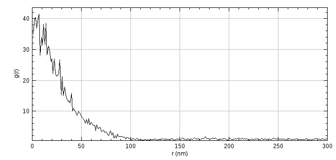
Fig. 7.1 Auto-correlation curve from PC-PALM analysis

7.3. PC-PALM Spatial Analysis

Perform pair-correlation spatial analysis as per the paper by [Puchnar, et al, 2013]. The method plots the molecule density around each localisation as a function of distance from the localisation.

Molecules representing distinct on bursts from a fluorophore over one or more frames must be prepared using PC-PALM Molecules. That plugin will create an image of the molecule data. A region of interest (ROI) can be marked on the image using any area ROI. This is the region that will be extracted from the molecule dataset for analysis. For example individual cells may be outlined using the freehand ROI tool. If no ROI is present then the plugin will analyse the entire dataset.

For each molecule in the analysis region a series of concentric rings is created from the centre up to a maximum distance. The number of surrounding molecules in each ring is counted and used to create a density plot against the radius.

Note that molecules within the maximum distance to the edge of the analysis region will have the outer concentric rings outside the region (i.e. they are clipped). This will reduce the density of these rings as no molecules can exist outside the analysis region. To avoid incorrect density figures any molecule within this border region can be excluded from the density analysis. This lowers the number of molecules analysed and ensures all molecules are surrounded by a complete density region. This option only correctly supports rectangular ROI. The distance from the edge of a freehand ROI is not correctly computed and some molecules may be included that have a clipped density region.

The following parameters are available:

Parameter	Description
Correlation distance	The maximum distance for the density analysis (in nm).
Use border	Set to true to skip density analysis for any molecule within the border region. The border is defined using the correlation distance inside the rectangular ROI bounds. This option will not correctly filter the border of non-rectangular freehand ROIs.
Correlation interval	The size of each concentric ring used for density counting (in nm).

When the analysis is complete the average density at each interval is displayed in a histogram (see Figure 7.2). Clustered data will show a peak at zero radius that falls away to a flat asymptote with increasing radius. The radius where the histogram is flat is a suitable radius to perform clustering to collect multiple occurrences of colocated molecules into clusters (see 7.7: PC-PALM Clusters). Note that if the input molecules have been previously clustered then the histogram can be used to check that clusters are uniformly distributed as the histogram for uniformly distributed data will be flat.

The density curve is saved in memory. Multiple curves can be combined using PC-PALM Fitting to create an aggregate curve from multiple datasets.

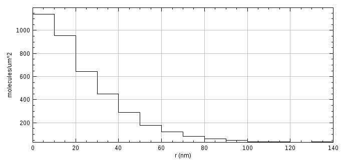
Fig. 7.2 Density histogram from PC-PALM spatial analysis

7.4. PC-PALM Save Results

Saves all the PC-PALM results held in memory to a results folder. When the plugin is run a folder must be selected. All results currently held in memory are saved to the folder in an XML format. Analysis results performed in the frequency domain to create a g(r) curve have the prefix Frequency; results performed in the spatial domain have the prefix Spatial.

7.5. PC-PALM Load Results

Loads all the PC-PALM results from a results folder to memory. When the plugin is run a folder must be selected. All files with the .xml suffix will be loaded. Each result file has an ID. The result will replace any current result held in memory with the same ID, otherwise the result will be added to the current results. To load results from different directories saved in different sessions of PC-PALM analysis (thus the IDs are not unique) requires editing the XML files to create a unique ID for each file.

An error is shown if any XML file is not recognised as a PC-PALM result.

7.6. PC-PALM Fitting

Combines multiple correlation curves calculated by PC-PALM Analysis into an average curve. The correlation curve from frequency domain analysis can be fit using various models.

Both the PC-PALM Analysis and PC-PALM Spatial Analysis plugins generate a curve with radial distance on the x axis. PC-PALM Analysis is done in the frequency domain following Fourier transform and produces an auto-correlation g(r) curve. PC-PALM Spatial Analysis is done in the spatial domain and produces a radial density curve. The curves are saved to memory and identified as either frequency domain or spatial domain curves.

When the PC-PALM Fitting plugin executes the source for the combined curve must be selected. The following options are available:

Input	Description
Load from file	Load a curve that has been previously saved by the PC-PALM Fitting plugin. If this option is selected a second dialog is presented to select the file.
Re-use previous curve	Re-use the most recent combined curve from a previous execution of the PC-PALM Fitting plugin. This option is to enable fitting and output settings for the plugin to be adjusted while using the same input curve. This is only available if a previous curve exists.
Select PC-PALM Analysis results	Select results saved to memory by the PC-PALM Analysis plugin. If this option is selected a second dialog is presented containing a list of available results. Results must be compatible so they can be combined. This requires the same pixel size and type of analysis. Those from a frequency analysis will be identified with a * after the result ID and the pixel size of the analysed image is displayed. Multiple results can be selected in the dialog. If the selected results are not from a compatible analysis then an error message is recorded to the ImageJ log. If only 1 results set is available then the dialog is skipped and the single result set selected.

Once the combined curve has been loaded the plugin plots the combined correlation curve and then presents analysis options. For a spatial domain curve the only option is to save the combined curve to file. For a frequency domain curve it is possible to fit the curve using models of different spatial distributions of data (see below).

7.6.1. Fitting the correlation curve

The models available are described in [Sengupta et al, 2011] and [Veatch, et al, 2012]. The curve is modelled as:

\[g(r)^\text{peaks} = g(r)^\text{stoch} + g(r)^\text{protein}\]

where \(g(r)^\text{peaks}\) is the correlation curve, \(g(r)^\text{stoch}\) represents the correlation observed for repeat occurrences of the same molecule due to blinking, and \(g(r)^\text{protein}\) represents the correlation that occurs due to association of different proteins, e.g. clustering.

Note repeat occurrences of the same molecule should be in the same position but are observed in different positions due to the uncertainty during the localisation process. Thus any data where the molecules are repeatedly observed will have a correlation at low radii due to repeat occurrences of the same position. This is modelled as:

\[g(r)^\text{stoch} = \frac{1}{4 \pi \sigma_s^2 \rho^\text{protein}} \exp(\frac{-r^2}{4 \sigma_s^2})\]

where \(\sigma_s\) is the average positional uncertainty in the molecule localisation and \(\rho^\text{protein}\) is the average protein density.

In the event of no association between proteins the molecules are uniform and the autocorrelation function of the protein molecules is 1. The autocorrelation function is as follows:

\[g(r)^\text{peaks} = g(r)^\text{stoch} + 1\]

If the proteins are distributed according to a micro-emulsion model the molecules will be randomly distributed within non-overlapping circles of a similar size (see Veatch et al (2012), figure 3). The micro-emulsion is modelled as:

\[g(r)^\text{protein} = \left( A \exp(\frac{-r}{\alpha}) \cos(\frac{\pi r}{2r_0}) + 1 \right) * g(r)^\text{PSF}\]

where \(A\) is an amplitude, \(\alpha\) is a measure of the coherence length between circles, \(r_0\) is the average circle radius and \(g(r)^\text{PSF}\) is the PSF of the imaging method due to the positional uncertainty of the molecule localisation:

\[g(r)^\text{PSF} = \frac{1}{4 \pi \sigma_s^2} \exp(\frac{-r^2}{4 \sigma_s^2})\]

The emulsion model distribution can be generated by the PC-PALM Molecules plugin simulation mode. Note that the damped cosine function is suitable when the observed correlation curve g(r) has a well defined dip below 1.

If the proteins are distributed in random clusters of no definite shape then the g(r) curve is modelled using an exponential:

\[g(r)^\text{protein} = \left( A \exp(\frac{-r}{\xi}) + 1 \right) * g(r)^\text{PSF}\]

where \(A\) is an amplitude, and \(\xi\) is proportional to the cluster size. The random cluster model distribution cannot be generated by the PC-PALM Molecules plugin simulation mode. The random cluster model allows expression of \(N^\text{cluster}\), the average occupancy of a cluster:

\[N^\text{cluster} = 2A \pi \xi^2 \rho^\text{protein}\]

The ratio of the density of the proteins in clusters to the average density across the entire image, i.e. the increased density of proteins in a cluster, is given by:

\[\psi^\text{cluster} = 2A\]

Note: Both the emulsion model and random clustered model (\(g(r)^\text{protein}\)) use a convolution of the protein model function with \(g(r)^\text{PSF}\). For simplicity the convolution can be omitted. This is valid when the positional uncertainty \(\sigma_s\) is an order of magnitude smaller than the spatial extent of clusters thus the Gaussian convolution has a small effect on the curve. Thus the emulsion model for \(g(r)^\text{protein}\) is a damped cosine function and the random clustered model is an exponential.

Fitting of the curve is performed using a least squares estimtor to minimise the difference between the g(r) curve and the model. The fit uses a bounded CMA-ES optimiser which is stochastic and derivative free. The initial solution may be improved if restarted and the number of restarts is configurable. Optionally an attempt can be made to improve the solution using a numerical gradient based method which is not suited to the initial search but works well when close to the optimal solution.

Note that the g(r) curve may have large errors when the radius r is low due to the positional uncertainty of the localisations. The plugin provides the option to ignore small r values when fitting the curve. The minimum r used is expressed as a factor of the estimated precision.

The curve is initially fit using the random model model and validated against the initial estimates. The fitted localisation precision and protein density are compared to the estimated precision and initial protein density (computed from the aggregated values output by PC-PALM Analysis for each g(r) curve). The change in the parameter is expressed as a percentage and the fit is rejected if above a threshold.

The random model is composed of the \(g(r)^\text{stoch} + 1\). If the stochastic component of the function is subtracted from the g(r) curve the value should be 1. If the value is above 1 then there is a \(g(r)^\text{protein}\) component in the curve not explained by the model. The random model fit can be rejected if the magnitude of the \(g(r)^\text{protein}\) component is above a threshold:

\[g(r)^\text{peaks} - g(r)^\text{stoch} > g(r)_\text{threshold}\]

If the random model is rejected then the plugin will apply the random clustered and emulsion clustered models to the data. The clustered models are again validated using the percentage change of the parameters from the initial estimates. The domain radius must be larger than the estimated localisation precision. The adjusted coefficient of determination is computed and the fit is rejected if the score does not improve and discourages overfitting using more complex models.

7.6.2. Parameters

The following parameters are available:

Parameter	Description
Estimated precision	The estimated positional uncertainty of the molecule localisation.
Blinking rate	The estimated average blinking rate of each fluorophore molecule.
Show error bars	Set to true show the standard error bars on the g(r) curve. This settings is relevant when the curve is an average composed from multiple input curves.
Fit restarts	The number of restarts to use for the bounded fitting process.
Refit using gradients	Set to true to refit from the initial solution using a gradient based method.
Fit above estimate precision	Ignore r) value on the *g(r) curve below N times the Estimated precision. This can be used to avoid the noisy part of the curve when fitting.
Fitting tolerance	Set the percentage tolerance for the difference between the fitted parameters and the initial estimates for localisation precision and protein density. If the fit changes the values by greater than this threshold the fit is rejected. Set to 0 to ignore fit validation.
gr random threshold	Set the threshold for the :math:`` component of the g(r) curve to reject the random model.
Fit clustered models	Set to true to always fit the clustered models. Otherwise only fit the clustered models if the random model is rejected.
Save correlation curve	Set to true to save the combined correlation curve to file. The file will also contain the curve data for each fitted model.

7.6.3. Results

Fitting details are recorded in the ImageJ log window. The fit for each model is displayed on the correlation curve plot. If low radius data was excluded from the fit using the Fit above estimate precision option then data points from the model below the distance threshold are shown using circles. The fit parameters are reported to a results table.

Field	Description
Model	The protein distribution model.
Colour	The colour of the model data points in the correlation curve plot.
Valid	Set to true if the model passed validation and, in the case of the clustered models, improved the fit of the random model.
Precision	The fitted precision \(\sigma_s\).
Density	The fitted protein density \(\rho^\text{protein}\).
Domain radius	For the clustered model the domain radius \(\xi\). For the emulsion model the average circle radius \(r_0\).
Domain Density	This is the amplitude component of \(g(r)^\text{protein}\), it is proportional to the density of proteins in the cluster.
N-cluster	For the clustered model the average occupancy of a cluster \(N^\text{cluster}\).
Coherence	For the emulsion clustered model the coherence length \(\alpha\).
Adjusted R2	The adjusted coefficient of determination.

7.7. PC-PALM Clusters

Clusters localisations using a distance threshold and produces a histogram of cluster size. This can be fit using a zero-truncated negative binomial distribution (with parameters n, p) to calculate the size of the clusters (n) and the probability of seeing a fluorophore (p).

The PC-PALM Clusters plugin is based on the paper by Puchnar, et al (2013). The analysis aims to determine the stoichiometry of colocated molecules, i.e. are closer than the localisation precision. Note that this is in contrast to the PC-PALM Fitting plugin which models clusters of molecules over distances in excess of the localisation precision. The analysis is based on two assumptions:

1. The activation, fluorescence and bleaching lifecycle for a fluorophore can be imaged without interference from other fluorophores.

2. The fluorophore activation probability is fixed.

The first assumption is that the activation of a single fluorophore, measurement of its location and its final photo-bleaching all occurs before another fluorophore at the same location is activated. This requires careful experimental conditions to avoid excess photoactivation and may also require separation of the photoactivation light from the readout light. In this case the readout light can be run for a long time until all photoactivity is reduced to background before the next round of photoactivation.

The second assumption is that the probability of a fluorophore being photoactivatable is fixed for all fluorophores in the imaging environment. Note that this is not the activation rate (the frequency of activations per second) but the probability that a fluorophore can be activated, for example it has avoided misfolding and the chromophore is valid.

An example of the analysis is to identify if a structure has a stoichiometry of 2 or 3 (dimer or trimer). An experiment is imaged so that all localisations at the same position within a set time span are from a single fluorophore; the fluorophore is then assumed to have bleached. Further localisations at the same positions are from a second fluorophore. This repeats for subsequent fluorophores. Clustering of the localisations within a time and distance threshold should collect all localisations from the same fluorophore into a single position. A second clustering of these molecules within a distance threshold should collect multimers together. A histogram of the count of N-mers would have a peak at 2 for dimers or 3 for trimers. Note however that not all fluorophores will be activated in the course of the entire experiment. If the activation probability is below 100% then a histogram of the counts for trimers would show some dimers (1 molecule not activated) and some monomers (2 molecules not activated). It is not possible to count the number of 0-mers; the histogram of N-mers thus shows a zero-truncated binomial distribution where the p-value is the probability of fluorophore activation.

The PC-PALM Molecules plugin can be used to cluster localisations with a distance and time threshold. This should collect all localisations from the same fluorophore into a single molecule. It is possible to demonstrate this using known monomers of the fluorophore randomly distributed on the image. The PC-PALM Spatial Analysis plugin produces a histogram of molecule density surrounding each molecule. When constructed using the raw localisations there will be a peak at low radii due to repeat occurrences of the same molecule. Where this peak reduces to a flat background is a suitable radius for clustering repeat localisations into molecules. If the monomer localisations are clustered using a suitable distance threshold they should be grouped into molecules; the histogram of molecule density surrounding each molecule should be flat. Performing the same clustering using uniformly spread N-mers would not show a flat histogram after clustering as the N-mers are colocated creating a peak in density close to the origin. The radius of this peak after the first clustering is a suitable radius for a second clustering that should collect the molecules of the N-mer together. The histogram of the cluster count (N) can be analysed to determine the stoichiometry of the N-mer.

Note: It is possible to simulate N-mers using the simulation mode of PC-PALM Molecules. The Blinking distribution parameter should be set to Binomial and the Blinking rate parameter is then the count (N) of the N-mer. The fluorophore activation probability can be configured. The Cluster simulation should be None to create a uniform distribution. This will create N-mers uniformly spread on the image.

The PC-PALM Clusters plugin provides fitting of a zero-truncated binomial distribution to a histogram of counts. The histogram can be loaded from file or created using clustering of the most recent molecules generated by PC-PALM Molecules. When the plugin runs a selection dialog is shown allowing the method to be specified: File or Clustering. If no molecules are present in memory then the dialog is not shown and the plugin defaults to file input. If clustering is performed then the histogram can be saved to allow it to be reloaded using the File option.

The histogram is fit for all N in a range and the p-value is optimised. The fit of each binomial(n,p) combination is scored using the residual sum of squares (SS). If the range for N is large then fitting will halt increasing N if no improvement is achieved for 3 consecutive increases in N. Fitting can use a least squares estimator (LSE) to minimise the SS or a maximum likelihood estimator (MLE). In the case of a MLE the score is the sum of the log-likelihood of the zero-truncated binomial distribution multiplied by the observed frequency:

\[\text{log-likelihood} = \sum\limits_{i=1}^n { \text{obs}_i * \ln( \text{B}(i|n, p)) }\]

where n is the target cluster size, and p is the current estimate for the p-value. Note that \(\text{B}(i|n, p)\) is zero when observations i is greater than the target n; this is valid for LSE but for MLE observations above the target n are ignored.

7.7.1. Noise subtraction

During an experiment there may be spurious background localisations. These can result in extra counts of molecules. These can be subtracted by performing the PC-PALM Clusters analysis on image data captured using the same imaging conditions but without fluorophores. This will create a histogram of molecules per cluster for background noise. The background noise can be subtracted from the histogram for the live experiment data.

The analysis is performed using the same settings for the live experiment on the background noise experiment. The histogram should be saved with a calibration (the number of frames and the area used for data capture).

The noise histogram can be subtracted from the live data histogram. When analysis is performed on a histogram the plugin will check if it is calibrated. This may be a calibrated histogram loaded from file or calibration added to a histogram created by clustering. If the histogram is calibrated the plugin will prompt the user if they wish to perform background subtraction. Additionally if the histogram was loaded from file an option will be provided to auto-save the noise subtracted histogram to file. The specified noise histogram is loaded. If the calibration units for the area match then the noise histogram is subtracted from the original histogram. Each histogram is converted from a raw counts histogram to counts per frame per area. The noise can then be subtracted from the live data. The remaining data is rescaled using the frames and area back to counts.

The noise subtracted histogram will be displayed in a new plot window. If auto-save was selected then the histogram is saved using the original input filename with the suffix updated to .noise.tsv.

Note: Clustering of molecules and background noise localisations produces higher counts than expected across the entire histogram. It is impossible to correctly subtract the additional high cluster counts due to noise. Experiments should be configured to minimise noise to the extent that noise localisations are unlikely to be colocated with localisations from fluorophores. The only significant contributions of noise localisations is a higher count of 1 molecule/cluster due to isolated noise localisations. In this situation background subtraction of noise mainly targets the count of monomers and can improve the fit of the binomial distribution to the corrected data.

7.7.2. Histogram normalisation

Histograms are calibrated using the number of frames (t) and the area of each frame (a). The counts (c) can be normalised using:

\[c_{norm} = \frac{c}{t a}\]

The counts per frame per area allows histograms from different experiments (with potentially different duration and imaging area) to be combined. Noise subtraction on a single histogram can be performed when loading a histogram from file. However combining histogram counts requires the experiments to be performed using very similar imaging conditions to avoid introducing artifacts in the summary histogram, for example due to vastly different number of observations between samples. Combination of histograms is not currently supported but can be done manually. Since each noise subtracted histogram should have the profile of the same binomial distribution, a combined histogram could be created by converting each histogram to sum to 1, averaging, then rescaling to a count; the combined histogram can be fit by the analysis plugin. Alternatively fitting could be performed simultaneously on multiple histograms in an external analysis package.

7.7.3. Parameters

The following parameters are available:

Parameter	Description
Distance	The clustering distance (in nm).
Algorithm	The clustering algorithm (see 6.3: Cluster Molecules).
Multi thread	Use multi-threading if available for the algorithm.
Weighted clustering	Set to true to use weighted clustering with each molecule weighted using the photon intensity. The weight effects the computation of the centre of mass of a cluster. The default is unweighted.
Min N	The minimum cluster size N to fit to the histogram.
Max N	The maximum cluster size N to fit to the histogram. Set to zero to use the maximum limit of the histogram data.
Show cumulative histogram	Set to true to show the cumulative histogram of the data. Each fit for the various cluster size N will be added to the plot.
Maximum likelihood.	Set to true to use maximum likelihood estimation (MLE); otherise using least squares estimation (LSE).
Save histogram	Set to true to save the histogram to file.
Calibrate histogram	Set to true to add a calibration to the histogram. The calibration is used to normalise the histogram counts to counts per frame per area. This allows histograms constructed from multiple datasets to be combined.
Frames	The number of frames used to generate the localisation data.
Area	The are of the region used to generate the localisation data.
Units	The units for the area.

Note: If the histogram is loaded from file many parameters are not applicable and will not be displayed in the dialog. The following parameters are available:

• Min N

• Max N

• Show cumulative histogram

• Maximum likelihood

7.7.4. Results

If clustering is performed the clusters are saved to memory using the name PC-PALM Clusters to allow analysis or export of the data with other plugins.

The histogram of the molecules per cluster is displayed (see Figure 7.3). Fitting details for each binomial distribution are recorded in the ImageJ log window. The best fit is recorded on the histogram using a magenta line. Note that the best fit line can include the expected count for zero molecules per cluster.

Optionally the cumulative probability histogram of molecules per cluster is displayed (see Figure 7.4). The fit for each binomial distribution is shown as a line (blue to red) and the best fit is recorded using a magenta line.

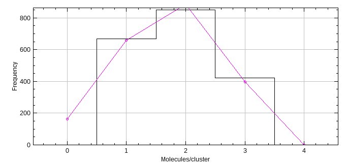
Fig. 7.3 Histogram of molecules per cluster from PC-PALM Clusters.

The data is from a simulation of trimers with an activation probability of 60%. The histogram is fit using a binomial distribution with different cluster size N. The best fit is shown as a magenta curve.

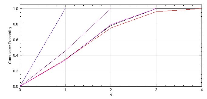
Fig. 7.4 Cumulative probability histogram of molecules per cluster from PC-PALM Clusters.

The data is from a simulation of trimers with an activation probability of 60%. The histogram is fit using a binomial distribution with different cluster size N. Each fit is shown using a coloured line from blue (lowest N) to red (highest N). The best fit is recorded on the histogram using a magenta line. The original curve is black with data points shown as circles.